Descriptive analysis of statistical associations with descriptio
Nicolas Robette
2024-03-07
Source:vignettes/articles/Article_eng.Rmd
Article_eng.Rmd
descriptio package provides some functions dedicated to
the description of statistical associations between variables. They are
based on effect size measures (also called association measures).
The main measures are built from simple concepts (correlations, proportion of variance explained), they are bounded (between -1 and 1 or between 0 and 1) and are not sensitive to the number of observations.
The main measures of global association are the following.
For the relationship between two categorical variables: the Cramér’s V which, unlike the chi-square, for example, is not sensitive to the number of observations or the number of categories of the variables. It varies between 0 (no association) and 1 (perfect association). Squared, it can be interpreted as the share of variation shared between two variables.
For the relationship between two numerical variables: Kendall’s (tau) or Spearman’s (rho) rank correlations, which detect monotonic relationships between variables, and not only linear ones as is the case with Pearson’s linear correlation. They vary between -1 and 1. An absolute value of 0 indicates no association, an absolute value of 1 a perfect association. The sign indicates the direction of the relationship.
For the relationship between a categorical variable and a numerical variable: the square of the correlation ratio (eta²). It expresses the proportion of the variance of the numerical variable “explained” by the categorical variable and varies between 0 and 1.
In addition to measures of global association, we also use measures of local association, i.e. at the level of the categories of the variables.
For the relationship between two categorical variables: the phi coefficient measures the attraction or repulsion in a cell of a contingency table. It varies between -1 and 1. An absolute value of 0 indicates an absence of association, an absolute value of 1 a perfect association. There is attraction if the sign is positive, repulsion if the sign is negative. Squared, phi is interpreted as the proportion of variance shared by the two binary variables associated with the categories studied. Unlike the test value, phi is not sensitive to the sample size.
For the relationship between a categorical variable and a numerical variable: the point biserial correlation measures the magnitude of the difference between the means of the numerical variable according to whether or not one belongs to the category studied. It varies between -1 and 1. An absolute value of 0 indicates no association, an absolute value of 1 a perfect association. The sign indicates the direction of the relationship. When squared, point biserial correlation can be interpreted as the proportion of variance of the numerical variable “explained” by the category of the categorical variable.
Note that if we code the categories of the categorical variables as binary variables with values of 0 or 1, the phi coefficient and the point biserial correlation are equivalent to Pearson’s correlation coefficient.
For more details on these effect size measurements, see: Rakotomalala
R., « Comprendre
la taille d’effet (effect size) »
In some functions of descriptio, association measures
can be completed by permutation tests, which are part
of combinatorial inference and constitute a
nonparametric alternative to the significance tests of
frequentist inference. A permutation test is performed in several
steps.
A measure of association between the two variables under study is computed.
The same measure of association is calculated from a “permuted” version of the data, i.e. by randomly “mixing” the values of one of the variables, in order to “break” the relationship between the variables.
Repeat step 2 a large number of times. This gives an empirical distribution (as opposed to the use of a theoretical distribution by frequentist inference) of the measure of association under the H0 hypothesis of no relationship between the two variables.
The result of step 1 is compared with the distribution obtained in 3. The p-value of the permutation test is the proportion of values of the H0 distribution that are more extreme than the measure of association observed in 1.
If all possible permutations are performed, the permutation test is
called “exact”. In practice, the computation time required is often too
important and only a part of the possible permutations is performed,
resulting in an “approximate” test. In the following examples, the
number of permutations is set to 100 to reduce the computation time, but
it is advisable to increase this number to obtain more accurate and
reliable results (for example nperm=1000).
To illustrate the statistical association analysis functions of
descriptio, we will use data on cinema. This is a sample of
1000 films released in France in the 2000s, for which we know the
budget, the genre, the country of origin, the “art et essai” label, the
selection in a festival (Cannes, Berlin or Venice), the average rating
of intellectual critics (according to Allociné) and the number of
admissions. Some of these variables are numerical, others are
categorical.
library(descriptio)
data(Movies)
str(Movies)
'data.frame':   1000 obs. of  7 variables:
 $ Budget   : num  3.10e+07 4.88e+06 3.50e+06 1.63e+08 2.17e+07 ...
 $ Genre    : Factor w/ 9 levels "Action","Animation",..: 1 5 7 1 7 5 1 7 5 7 ...
 $ Country  : Factor w/ 4 levels "Europe","France",..: 4 2 2 1 2 2 4 4 2 4 ...
 $ ArtHouse : Factor w/ 2 levels "No","Yes": 1 1 2 1 2 1 1 1 1 1 ...
 $ Festival : Factor w/ 2 levels "No","Yes": 1 1 1 1 1 1 1 1 1 1 ...
 $ Critics  : num  3 1 3.75 3.75 3.6 2.75 1 1 1 3 ...
 $ BoxOffice: num  1013509 24241 39376 6996996 493416 ...
Relationship between two variables
The package offers several functions to study the statistical relationship between two variables, depending on the nature (categorical or numerical) of these variables.
Two categorical variables
The function assoc_twocat computes :
- the contingency table (numbers)
- the percentages, the row-percentages and the column-percentages
- the theoretical numbers, i.e. in a situation of independence
- the chi-square
- the Cramér’s V and the p-value of the corresponding permutation test
- the Goodman & Kruskal tau (an asymetrical measure of association)
- the Pearson residuals, adjusted or not
- the odds ratios for every cell of the contingency table
- the phi coefficients and the p-values of the corresponding permutation tests
- the global and local PEMs (Percentage of Maximum Deviation from Independence, see Cibois 1993)
- a summary table of these results
res <- assoc.twocat(Movies$Country, Movies$ArtHouse, nperm=100)
res$tables
$freq
         No  Yes  Sum
Europe   39   33   72
France  212  393  605
Other     6   20   26
USA     257   40  297
Sum     514  486 1000

$prop
          No   Yes   Sum
Europe   3.9   3.3   7.2
France  21.2  39.3  60.5
Other    0.6   2.0   2.6
USA     25.7   4.0  29.7
Sum     51.4  48.6 100.0

$rprop
             No      Yes Sum
Europe 54.16667 45.83333 100
France 35.04132 64.95868 100
Other  23.07692 76.92308 100
USA    86.53199 13.46801 100
Sum    51.40000 48.60000 100

$cprop
               No        Yes   Sum
Europe   7.587549   6.790123   7.2
France  41.245136  80.864198  60.5
Other    1.167315   4.115226   2.6
USA     50.000000   8.230453  29.7
Sum    100.000000 100.000000 100.0

$expected
            No     Yes
Europe  37.008  34.992
France 310.970 294.030
Other   13.364  12.636
USA    152.658 144.342
res$global
$chi.squared
[1] 220.1263

$cramer.v
[1] 0.4691762

$permutation.pvalue
[1] 0

$global.pem
[1] 64.04814

$GK.tau.xy
[1] 0.2201263

$GK.tau.yx
[1] 0.1537807
res$local
$std.residuals
               No        Yes
Europe  0.3274474 -0.3367479
France -5.6123445  5.7717531
Other  -2.0143992  2.0716146
USA     8.4449945 -8.6848595

$adj.residuals
               No        Yes
Europe   0.487584  -0.487584
France -12.809366  12.809366
Other   -2.927844   2.927844
USA     14.447862 -14.447862

$adj.res.pval
                No         Yes
Europe 0.625844564 0.625844564
France 0.000000000 0.000000000
Other  0.003413213 0.003413213
USA    0.000000000 0.000000000

$odds.ratios
               No        Yes
Europe  1.1270813  0.8872474
France  0.1661190  6.0197809
Other   0.2751969  3.6337625
USA    11.1500000  0.0896861

$local.pem
        y
x               No       Yes
  Europe   5.69273  -5.69273
  France -51.55493  51.55493
  Other  -55.10326  55.10326
  USA     72.28804 -72.28804

$phi
                No         Yes
Europe  0.01541876 -0.01541876
France -0.40506773  0.40506773
Other  -0.09258656  0.09258656
USA     0.45688150 -0.45688150

$phi.perm.pval
                 No          Yes
Europe 2.809065e-01 2.809065e-01
France 2.012492e-41 0.000000e+00
Other  5.935146e-04 5.935146e-04
USA    0.000000e+00 2.285184e-49
res$gather
  var.y  var.x freq  prop     rprop      cprop expected std.residuals adj.residuals         or       pem         phi    perm.pval freq.x freq.y prop.x prop.y
1    No Europe   39 0.039 0.5416667 0.07587549   37.008     0.3274474      0.487584  1.1270813   5.69273  0.01541876 2.809065e-01     72    514  0.072  0.514
2    No France  212 0.212 0.3504132 0.41245136  310.970    -5.6123445    -12.809366  0.1661190 -51.55493 -0.40506773 2.012492e-41    605    514  0.605  0.514
3    No  Other    6 0.006 0.2307692 0.01167315   13.364    -2.0143992     -2.927844  0.2751969 -55.10326 -0.09258656 5.935146e-04     26    514  0.026  0.514
4    No    USA  257 0.257 0.8653199 0.50000000  152.658     8.4449945     14.447862 11.1500000  72.28804  0.45688150 0.000000e+00    297    514  0.297  0.514
 [ reached 'max' / getOption("max.print") -- omitted 4 rows ]
The function ggassoc_crosstab presents the contingency
table in graphical form, with rectangles whose area corresponds to the
number of observations and whose color gradient corresponds to the
attraction/repulsion (from one of the local association measures
proposed in assoc.twocat, here the phi coefficients). The
“art et essai” label is clearly over-represented among French films and
under-represented among American films.
ggassoc_crosstab(Movies, ggplot2::aes(x=Country, y=ArtHouse))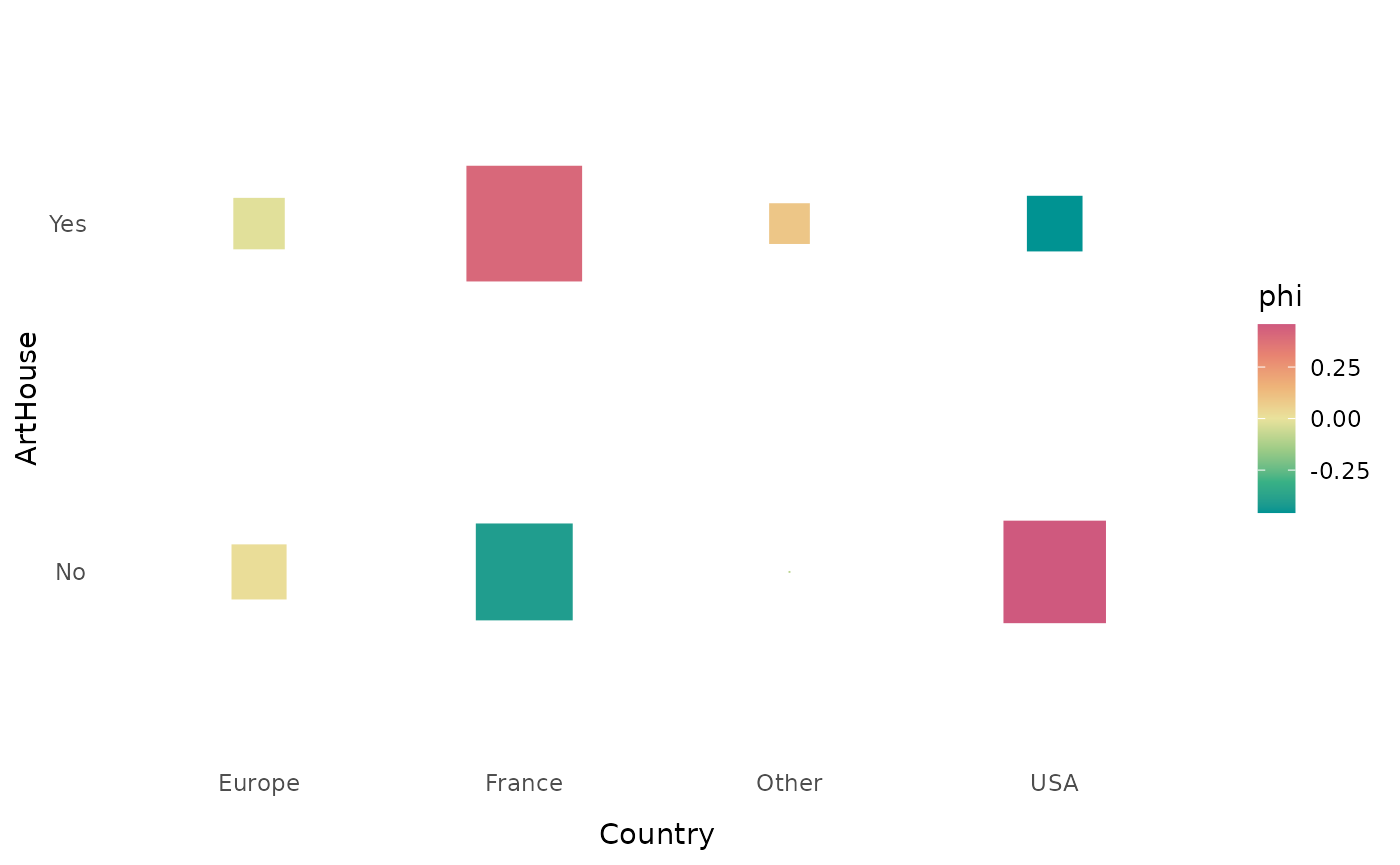
The function ggassoc_phiplot proposes another way to
represent the attractions/repulsions. The width of the rectangles
corresponds to the numbers of the variable x, their height to the local
associations (by default phi coefficients). The rectangles are colored
in black when there is attraction, in white when there is repulsion.
ggassoc_phiplot(Movies, ggplot2::aes(x=Country, y=ArtHouse))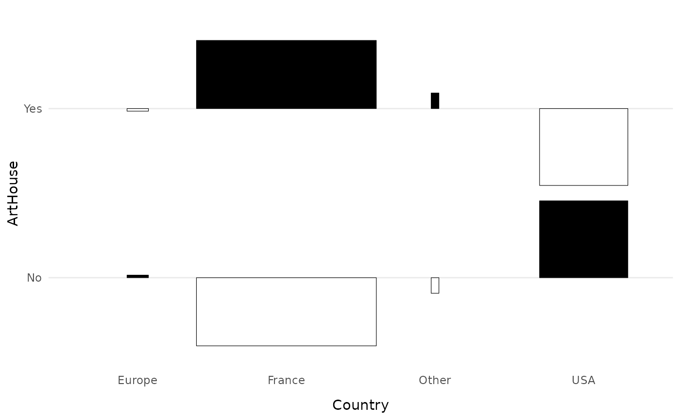
The function ggassoc_bertin is inspired by Jacques
Bertin’s principles of graphical semiology for the representation of a
data matrix and by the tool AMADO
Online. The height of the bars corresponds to the conditional
probabilities of y given x. They are colored black when the conditional
probabilities are greater than the marginal probabilities of y. The
width of the bars can be adjusted to be proportional to the marginal
probabilities of x.
ggassoc_bertin(Movies, ggplot2::aes(x=Country, y=ArtHouse), prop.width = TRUE, add.gray = TRUE)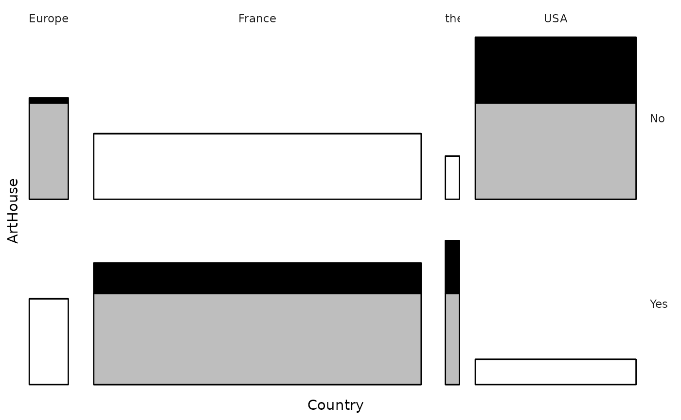
The function ggassoc_assocplot produces an “association
plot” as proposed by Cohen (1980) and Friendly (1992). The width of the
bars is proportional to the square root of the theoretical numbers. The
height of the bars and the color gradient are proportional to the local
associations. If these local associations are measured by Pearson
residuals (the default choice), the area of the bars is proportional to
the difference between the theoretical and observed numbers.
When the number of categories of the variables is high, as here when we cross the genre of the film and its geographical origin, it can be useful to sort the rows and/or the columns so that those which are similar are close.
We see that action, animation, science fiction and horror films are over-represented among American films, and that documentaries, dramas and comedy-dramas are over-represented among French films.
ggassoc_assocplot(Movies, ggplot2::aes(x=Country, y=Genre), sort = "both")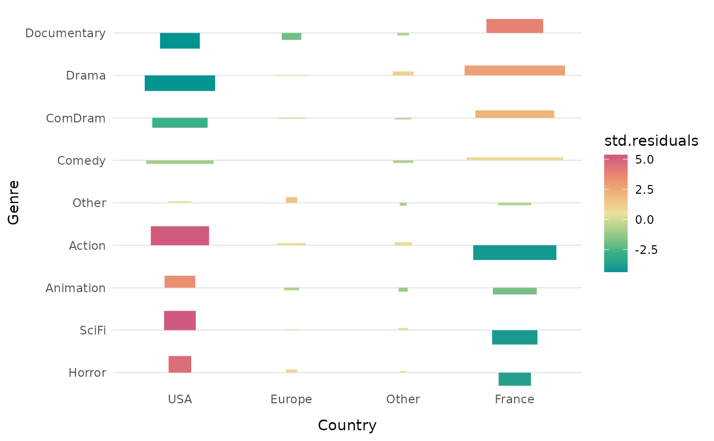
The function ggassoc_chiasmogram draws a “chiasmogram”,
a graphical representation proposed by Bozon and Héran (1988). The width
of the rectangles is proportional to the marginal probabilities of the
variable in column, their height is proportional to the marginal
probabilities of the variable in row. The surface area of the rectangles
is therefore proportional to the theoretical numbers. The rectangles are
colored according to the degree of local association (by default the phi
coefficients).
ggassoc_chiasmogram(Movies, ggplot2::aes(x=Country, y=Genre), sort = "both")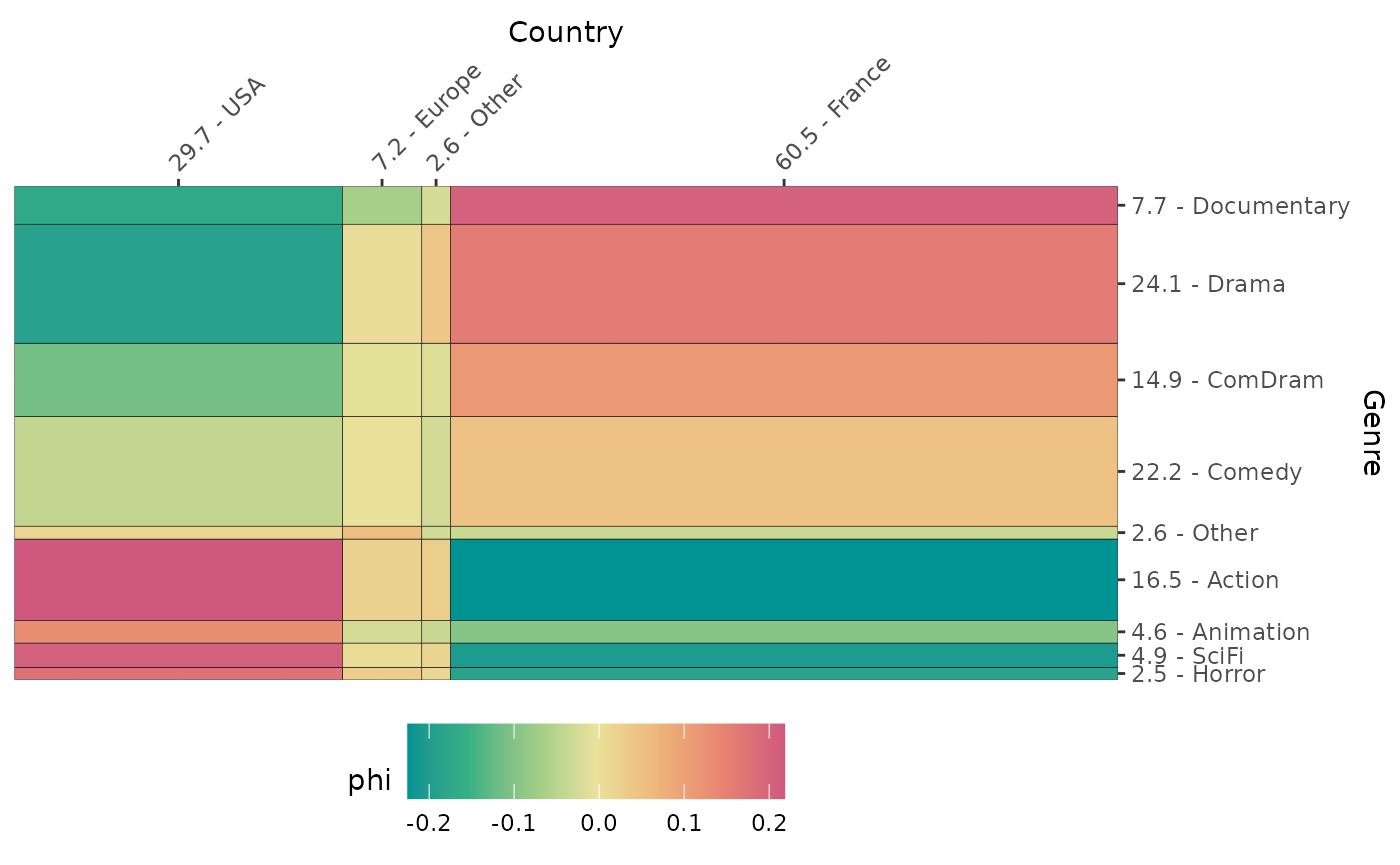
The function ggassoc_marimekko produces marimekko
charts, also called mosaic plots. The width of the bars is proportional
to the marginal probabilities of the variable x, their height to the
conditional probabilities of the variable y given x.
ggassoc_marimekko(Movies, ggplot2::aes(x=Country, y=Genre), sort = "both", type = "classic")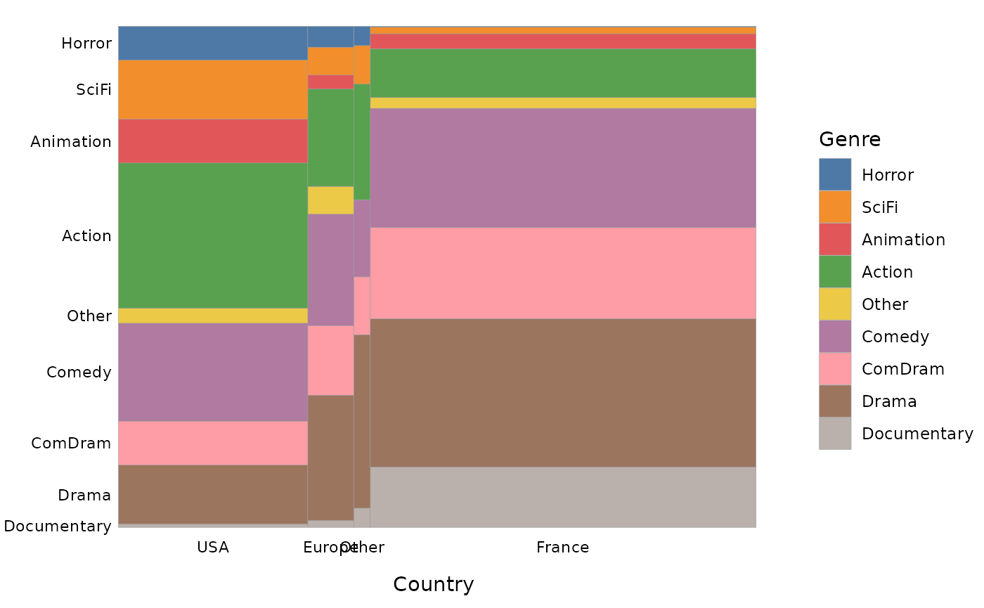
We can choose to color the bars according to the degree of local association (here the phi coefficients), as proposed by Friendly (1994).
ggassoc_marimekko(Movies, ggplot2::aes(x=Country, y=Genre), sort = "both", type = "shades")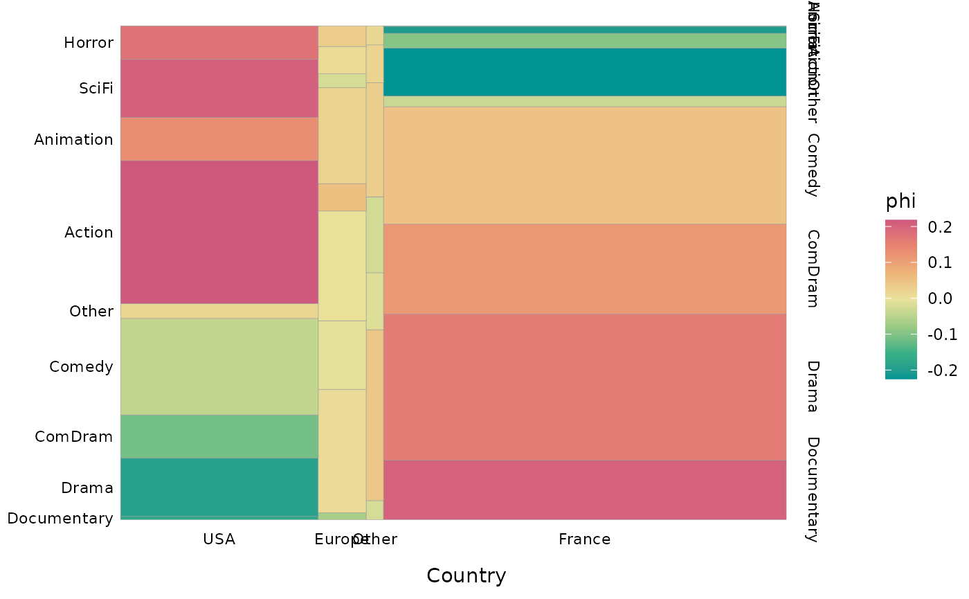
We can also choose to replace the gradient of colors by textures more or less dense according to the degree of local association.
ggassoc_marimekko(Movies, ggplot2::aes(x=Country, y=Genre), sort = "both", type = "patterns")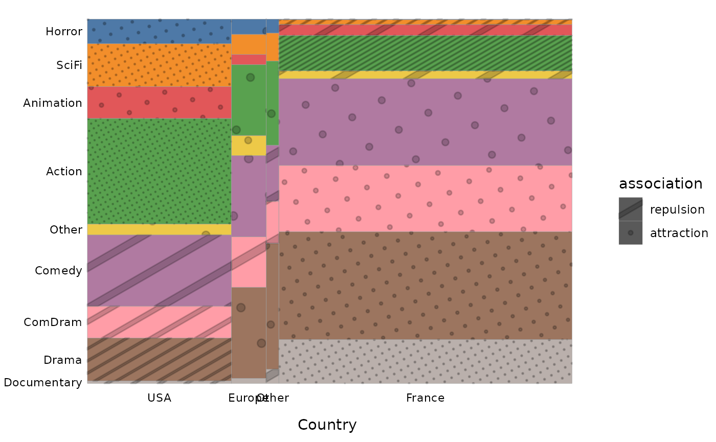
One categorical variable and one numerical variable
The assoc_catcont function computes:
- the squared correlation ratio (eta²) and the p-value of the corresponding permutation test
- the point biserial correlations and the p-values of the corresponding permutation tests
assoc.catcont(Movies$Country, Movies$Critics, nperm=100)
$summary
           mean        sd min       q1   median   q3      max       mad
Europe 2.886343 0.7328983 1.4 2.458333 3.000000 3.40 4.833333 0.5000000
France 2.923361 0.8469909 1.0 2.333333 3.000000 3.50 5.000000 0.6000000
Other  3.041026 0.8039995 1.0 2.425000 3.208333 3.65 4.400000 0.6000000
USA    2.686700 0.8601259 1.0 2.000000 2.666667 3.20 5.000000 0.6666667

$eta.squared
[1] 0.0169216

$permutation.pvalue
[1] 5.722966e-08

$cor
Europe France  Other    USA
 0.011  0.102  0.036 -0.128

$cor.perm.pval
      Europe       France        Other          USA
3.640301e-01 9.229488e-04 1.444155e-01 8.836613e-05

$test.values
   Europe    France     Other       USA
 0.340764  3.218873  1.140324 -4.033595

$test.values.pval
      Europe       France        Other          USA
7.332813e-01 1.286957e-03 2.541511e-01 5.492984e-05
The function ggassoc_boxplot represents the relationship
between the variables in the form of box-plots and/or “violin”
distributions.
ggassoc_boxplot(Movies, ggplot2::aes(x=Country, y=Critics))Two numerical variables
The function assoc_twocont computes the Kendall and
Spearman rank correlations and the Pearson linear correlation, as well
as the p-values of the corresponding permutation tests.
assoc.twocont(Movies$Budget, Movies$BoxOffice, nperm=100)
                     pearson  spearman   kendall
value              0.6053018 0.7084613 0.5184719
permutation.pvalue 0.0000000 0.0000000 0.0000000
The function ggassoc_scatter represents the relationship
between the two variables in the form of a scatterplot, with an
approximation by smoothing (with the “Generalized Additive Model”
method).
ggassoc_scatter(Movies, ggplot2::aes(x=Budget, y=BoxOffice))Relationships between one variable Y and a set of variables X
Often, not just two variables are studied, but a larger set of
variables. When one of these variables has the status of an “explained”
variable, one generally uses regression models or, possibly, supervised
learning models (see the vignette of the moreparty package
for an example). However, it is essential to know all the bivariate
relations of the dataset before moving to an “all else being equal”
approach.
It should be noted that if we do this work in a meticulous way,
adding eventually the descriptive analysis of the relationships between
three or four variables, we often realize that the surplus of knowledge
brought by the regression models is quite limited.
The function assoc.yx computes the global association
between Y and each of the variables of X, and for all pairs of variables
of X.
assoc.yx(Movies$BoxOffice, Movies[,-7], nperm=10)
$YX
  variable     measure association permutation.pvalue
1    Genre        Eta2       0.173              0.000
2 ArtHouse        Eta2       0.075              0.000
3  Country        Eta2       0.048              0.000
4   Budget Kendall tau       0.518              0.000
5  Critics Kendall tau       0.006              0.522
6 Festival        Eta2       0.000              0.885

$XX
   variable1 variable2     measure association permutation.pvalue
1      Genre  ArtHouse    Cramer V       0.554              0.000
2    Country  ArtHouse    Cramer V       0.469              0.000
3      Genre   Country    Cramer V       0.275              0.000
4   ArtHouse  Festival    Cramer V       0.229              0.000
5     Budget   Country        Eta2       0.287              0.000
6     Budget     Genre        Eta2       0.281              0.000
7   ArtHouse   Critics        Eta2       0.236              0.000
8     Budget  ArtHouse        Eta2       0.181              0.000
9      Genre   Critics        Eta2       0.090              0.000
10  Festival   Critics        Eta2       0.041              0.000
11    Budget   Critics Kendall tau      -0.178              0.000
12     Genre  Festival    Cramer V       0.183              0.000
13   Country   Critics        Eta2       0.017              0.000
14    Budget  Festival        Eta2       0.003              0.088
15   Country  Festival    Cramer V       0.035              0.671
The functions catdesc and condesc allow to go
into more detail about the relationships, by going to the category
level.
catdesc deals with the cases where Y is a categorical
variable. For a categorical variable X1, it computes, for a given
category of Y and a category of X1 :
- the percentage of the category of Y in the category of X1
- the percentage of the X1 category in the Y category
- the percentage of the X1 category in the whole sample
- the local association (by default the phi coefficient)
The results are sorted by decreasing local association and can be filtered to keep only the associations above a given threshold (in absolute value).
For a numerical variable X2, for a given category of Y, it computes :
- the median of X2 in the category of Y
- the median of X2 in the whole sample
- the dispersion of X2 in the Y category
- the dispersion of X2 in the whole sample
- the point biserial correlation
Dispersion is measured by the “median absolute deviation” (MAD), which is the median of the absolute deviations from the median. The median and MAD are so-called “robust” indicators, i.e. not sensitive to outliers, but one can choose to use the mean and standard deviation instead.
res <- catdesc(Movies$Festival, Movies[,-5], nperm = 10)
res$bylevel$Yes
$categories
       categories freq pct.y.in.x pct.x.in.y overall.pct.x    phi  pvalue
1    ArtHouse.Yes   68       14.0       88.3          48.6  0.229 0.00000
2     Genre.Drama   36       14.9       46.8          24.1  0.153 0.00000
3     Genre.Other    3       11.5        3.9           2.6  0.024 0.07162
4  Country.Europe    7        9.7        9.1           7.2  0.021 0.37955
5  Country.France   49        8.1       63.6          60.5  0.019 0.32078
6   Genre.ComDram   13        8.7       16.9          14.9  0.016 0.08648
7    Genre.Action   13        7.9       16.9          16.5  0.003 0.37480
8   Country.Other    2        7.7        2.6           2.6  0.000 0.43136
9     Genre.SciFi    3        6.1        3.9           4.9 -0.013 0.29380
10    Country.USA   19        6.4       24.7          29.7 -0.032 0.25998
 [ reached 'max' / getOption("max.print") -- omitted 5 rows ]

$continuous.var
  variables median.in.category overall.median mad.in.category overall.mad correlation  pvalue
1   Critics                3.5            3.0            0.67         0.6       0.204 0.00000
2 BoxOffice           198796.0       107326.5       181590.00    104060.0       0.008 0.27718
3    Budget          7000000.0      6127500.0      4438000.00   5156921.0      -0.057 0.00999
condesc deals with the cases where Y is a numerical
variable. For a categorical variable X1, it computes :
- the median of Y in the category of X1
- the median of Y in the whole sample
- the dispersion of Y in the category of X1
- the dispersion of Y in the whole sample
- the point biserial correlation
The results are sorted by decreasing point biserial correlation and can be filtered to keep only associations above a given threshold (in absolute value).
For the numerical variables of X, it calculates the correlation (by default Kendall’s tau).
condesc(Movies$BoxOffice, Movies[,-7], nperm=100)
$variables
  variable     measure association  pvalue
1    Genre        Eta2       0.173 0.00000
2 ArtHouse        Eta2       0.075 0.00000
3  Country        Eta2       0.048 0.00000
4   Budget Kendall tau       0.518 0.00000
5  Critics Kendall tau       0.006 0.38534
6 Festival        Eta2       0.000 0.76985

$categories
        categories median.in.category overall.median mad.in.category overall.mad correlation  pvalue
1      Genre.SciFi           680900.0       107326.5        607448.0      104060       0.294 0.00000
2      ArtHouse.No           264200.0       107326.5        232183.0      104060       0.274 0.00000
3  Genre.Animation           668896.0       107326.5        633265.0      104060       0.211 0.00000
4      Country.USA           328559.0       107326.5        274892.0      104060       0.192 0.00000
5     Genre.Action           240080.0       107326.5        202793.0      104060       0.087 0.00230
6   Country.Europe           108121.5       107326.5        104606.5      104060       0.068 0.00361
7     Festival.Yes           198796.0       107326.5        181590.0      104060       0.008 0.45057
8     Genre.Comedy           202090.0       107326.5        191819.0      104060       0.004 0.44342
9      Genre.Other           186084.5       107326.5        171739.5      104060      -0.005 0.41612
10     Festival.No           102726.0       107326.5         99642.0      104060      -0.008 0.43075
 [ reached 'max' / getOption("max.print") -- omitted 7 rows ]
The darma function presents the results in a form close to
that of a table of results of a regression.
When the variable Y is numerical, the function computes :
- for numerical X variables, the correlation (by deafult Kendall’s tau) and the p-value of the corresponding permutation test
- for the categories of the categorical X variables, the median of Y in the category, the point biserial correlation and the p-value of the corresponding permutation test
res <- darma(Movies$BoxOffice, Movies[,-7], nperm=10)| variable | measure | association | pvalue |
|---|---|---|---|
| ArtHouse | Cramer V | 0.229 | 0.00000 |
| Critics | Eta2 | 0.041 | 0.00000 |
| Genre | Cramer V | 0.183 | 0.00000 |
| Budget | Eta2 | 0.003 | 0.00000 |
| Country | Cramer V | 0.035 | 0.68387 |
| BoxOffice | Eta2 | 0.000 | 0.75176 |
| categories | freq | pct.y.in.x | pct.x.in.y | overall.pct.x | phi | pvalue |
|---|---|---|---|---|---|---|
| ArtHouse.No | 505 | 98.2 | 54.7 | 51.4 | 0.229 | 0.00000 |
| Genre.Comedy | 216 | 97.3 | 23.4 | 22.2 | 0.100 | 0.00189 |
| Genre.Documentary | 75 | 97.4 | 8.1 | 7.7 | 0.055 | 0.00530 |
| Genre.Horror | 25 | 100.0 | 2.7 | 2.5 | 0.046 | 0.06221 |
| Genre.Animation | 45 | 97.8 | 4.9 | 4.6 | 0.046 | 0.13446 |
| Country.USA | 278 | 93.6 | 30.1 | 29.7 | 0.032 | 0.25998 |
| Genre.SciFi | 46 | 93.9 | 5.0 | 4.9 | 0.013 | 0.29380 |
| Country.Other | 24 | 92.3 | 2.6 | 2.6 | 0.000 | 0.43136 |
| Genre.Action | 152 | 92.1 | 16.5 | 16.5 | -0.003 | 0.37480 |
| Genre.ComDram | 136 | 91.3 | 14.7 | 14.9 | -0.016 | 0.08648 |
| Country.France | 556 | 91.9 | 60.2 | 60.5 | -0.019 | 0.32078 |
| Country.Europe | 65 | 90.3 | 7.0 | 7.2 | -0.021 | 0.37955 |
| Genre.Other | 23 | 88.5 | 2.5 | 2.6 | -0.024 | 0.07162 |
| Genre.Drama | 205 | 85.1 | 22.2 | 24.1 | -0.153 | 0.00000 |
| ArtHouse.Yes | 418 | 86.0 | 45.3 | 48.6 | -0.229 | 0.00000 |
| variables | median.in.category | overall.median | mad.in.category | overall.mad | correlation | pvalue |
|---|---|---|---|---|---|---|
| Budget | 6034248.0 | 6127500.0 | 5160544.0 | 5156921.0 | 0.057 | 0.00008 |
| BoxOffice | 102726.0 | 107326.5 | 99642.0 | 104060.0 | -0.008 | 0.29523 |
| Critics | 2.8 | 3.0 | 0.6 | 0.6 | -0.204 | 0.00000 |
| categories | freq | pct.y.in.x | pct.x.in.y | overall.pct.x | phi | pvalue |
|---|---|---|---|---|---|---|
| ArtHouse.Yes | 68 | 14.0 | 88.3 | 48.6 | 0.229 | 0.00000 |
| Genre.Drama | 36 | 14.9 | 46.8 | 24.1 | 0.153 | 0.00000 |
| Genre.Other | 3 | 11.5 | 3.9 | 2.6 | 0.024 | 0.07162 |
| Country.Europe | 7 | 9.7 | 9.1 | 7.2 | 0.021 | 0.37955 |
| Country.France | 49 | 8.1 | 63.6 | 60.5 | 0.019 | 0.32078 |
| Genre.ComDram | 13 | 8.7 | 16.9 | 14.9 | 0.016 | 0.08648 |
| Genre.Action | 13 | 7.9 | 16.9 | 16.5 | 0.003 | 0.37480 |
| Country.Other | 2 | 7.7 | 2.6 | 2.6 | 0.000 | 0.43136 |
| Genre.SciFi | 3 | 6.1 | 3.9 | 4.9 | -0.013 | 0.29380 |
| Country.USA | 19 | 6.4 | 24.7 | 29.7 | -0.032 | 0.25998 |
| Genre.Animation | 1 | 2.2 | 1.3 | 4.6 | -0.046 | 0.13446 |
| Genre.Horror | 0 | 0.0 | 0.0 | 2.5 | -0.046 | 0.06221 |
| Genre.Documentary | 2 | 2.6 | 2.6 | 7.7 | -0.055 | 0.00530 |
| Genre.Comedy | 6 | 2.7 | 7.8 | 22.2 | -0.100 | 0.00189 |
| ArtHouse.No | 9 | 1.8 | 11.7 | 51.4 | -0.229 | 0.00000 |
| variables | median.in.category | overall.median | mad.in.category | overall.mad | correlation | pvalue |
|---|---|---|---|---|---|---|
| Critics | 3.5 | 3.0 | 0.67 | 0.6 | 0.204 | 0.00000 |
| BoxOffice | 198796.0 | 107326.5 | 181590.00 | 104060.0 | 0.008 | 0.27718 |
| Budget | 7000000.0 | 6127500.0 | 4438000.00 | 5156921.0 | -0.057 | 0.00999 |
When the variable Y is categorical, the function computes :
- for numerical X variables, the point biserial correlation and the p-value of the corresponding permutation test
- for the categories of the categorical X variables, the percentage of Y in the category, the phi coefficient and the p-value of the corresponding permutation test.
res <- darma(Movies$Festival, Movies[,-5], target=2, nperm=10)| variable | measure | association | pvalue |
|---|---|---|---|
| ArtHouse | Cramer V | 0.229 | 0.00000 |
| Critics | Eta2 | 0.041 | 0.00000 |
| Genre | Cramer V | 0.183 | 0.00000 |
| Budget | Eta2 | 0.003 | 0.00000 |
| Country | Cramer V | 0.035 | 0.68387 |
| BoxOffice | Eta2 | 0.000 | 0.75176 |
| categories | freq | pct.y.in.x | pct.x.in.y | overall.pct.x | phi | pvalue |
|---|---|---|---|---|---|---|
| ArtHouse.No | 505 | 98.2 | 54.7 | 51.4 | 0.229 | 0.00000 |
| Genre.Comedy | 216 | 97.3 | 23.4 | 22.2 | 0.100 | 0.00189 |
| Genre.Documentary | 75 | 97.4 | 8.1 | 7.7 | 0.055 | 0.00530 |
| Genre.Horror | 25 | 100.0 | 2.7 | 2.5 | 0.046 | 0.06221 |
| Genre.Animation | 45 | 97.8 | 4.9 | 4.6 | 0.046 | 0.13446 |
| Country.USA | 278 | 93.6 | 30.1 | 29.7 | 0.032 | 0.25998 |
| Genre.SciFi | 46 | 93.9 | 5.0 | 4.9 | 0.013 | 0.29380 |
| Country.Other | 24 | 92.3 | 2.6 | 2.6 | 0.000 | 0.43136 |
| Genre.Action | 152 | 92.1 | 16.5 | 16.5 | -0.003 | 0.37480 |
| Genre.ComDram | 136 | 91.3 | 14.7 | 14.9 | -0.016 | 0.08648 |
| Country.France | 556 | 91.9 | 60.2 | 60.5 | -0.019 | 0.32078 |
| Country.Europe | 65 | 90.3 | 7.0 | 7.2 | -0.021 | 0.37955 |
| Genre.Other | 23 | 88.5 | 2.5 | 2.6 | -0.024 | 0.07162 |
| Genre.Drama | 205 | 85.1 | 22.2 | 24.1 | -0.153 | 0.00000 |
| ArtHouse.Yes | 418 | 86.0 | 45.3 | 48.6 | -0.229 | 0.00000 |
| variables | median.in.category | overall.median | mad.in.category | overall.mad | correlation | pvalue |
|---|---|---|---|---|---|---|
| Budget | 6034248.0 | 6127500.0 | 5160544.0 | 5156921.0 | 0.057 | 0.00008 |
| BoxOffice | 102726.0 | 107326.5 | 99642.0 | 104060.0 | -0.008 | 0.29523 |
| Critics | 2.8 | 3.0 | 0.6 | 0.6 | -0.204 | 0.00000 |
| categories | freq | pct.y.in.x | pct.x.in.y | overall.pct.x | phi | pvalue |
|---|---|---|---|---|---|---|
| ArtHouse.Yes | 68 | 14.0 | 88.3 | 48.6 | 0.229 | 0.00000 |
| Genre.Drama | 36 | 14.9 | 46.8 | 24.1 | 0.153 | 0.00000 |
| Genre.Other | 3 | 11.5 | 3.9 | 2.6 | 0.024 | 0.07162 |
| Country.Europe | 7 | 9.7 | 9.1 | 7.2 | 0.021 | 0.37955 |
| Country.France | 49 | 8.1 | 63.6 | 60.5 | 0.019 | 0.32078 |
| Genre.ComDram | 13 | 8.7 | 16.9 | 14.9 | 0.016 | 0.08648 |
| Genre.Action | 13 | 7.9 | 16.9 | 16.5 | 0.003 | 0.37480 |
| Country.Other | 2 | 7.7 | 2.6 | 2.6 | 0.000 | 0.43136 |
| Genre.SciFi | 3 | 6.1 | 3.9 | 4.9 | -0.013 | 0.29380 |
| Country.USA | 19 | 6.4 | 24.7 | 29.7 | -0.032 | 0.25998 |
| Genre.Animation | 1 | 2.2 | 1.3 | 4.6 | -0.046 | 0.13446 |
| Genre.Horror | 0 | 0.0 | 0.0 | 2.5 | -0.046 | 0.06221 |
| Genre.Documentary | 2 | 2.6 | 2.6 | 7.7 | -0.055 | 0.00530 |
| Genre.Comedy | 6 | 2.7 | 7.8 | 22.2 | -0.100 | 0.00189 |
| ArtHouse.No | 9 | 1.8 | 11.7 | 51.4 | -0.229 | 0.00000 |
| variables | median.in.category | overall.median | mad.in.category | overall.mad | correlation | pvalue |
|---|---|---|---|---|---|---|
| Critics | 3.5 | 3.0 | 0.67 | 0.6 | 0.204 | 0.00000 |
| BoxOffice | 198796.0 | 107326.5 | 181590.00 | 104060.0 | 0.008 | 0.27718 |
| Budget | 7000000.0 | 6127500.0 | 4438000.00 | 5156921.0 | -0.057 | 0.00999 |
Relationships between all variables in a set
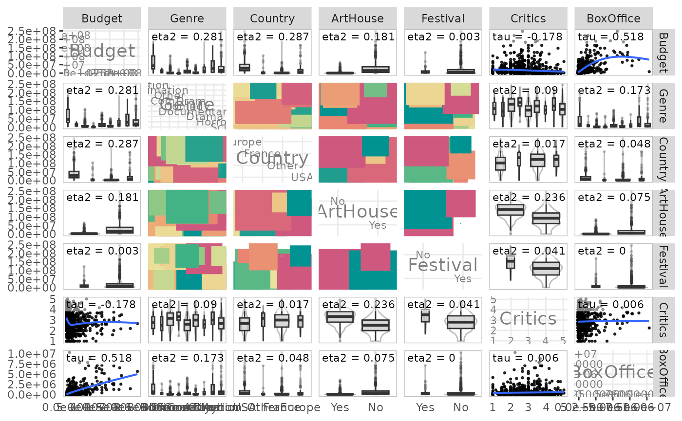
Finally, the ggassoc_* functions are designed to be
integrated in the plot matrices of the GGally package.
It is thus possible to use them to represent in a single plot all the
bivariate relations of a group of variables.
library(GGally)
ggpairs(Movies,
        lower = list(continuous = ggassoc_scatter,
                     combo = ggassoc_boxplot,
                     discrete = ggassoc_crosstab),
        upper = list(continuous = ggassoc_scatter,
                     combo = ggassoc_boxplot,
                     discrete = ggassoc_crosstab),
        diag = list(continuous = wrap("diagAxis", gridLabelSize = 3),
                           discrete = wrap("diagAxis", gridLabelSize = 3)))