Density plot of a supplementary variable

For a given category of a supplementary variable, adds a layer representing the density of points to the cloud of individuals, either with contours or areas.

ggadd_density(p, resmca, var, cat = levels(var)[1], axes = c(1,2),
density = "contour", col.contour = "darkred", pal.area = "viridis",
alpha.area = 0.2, ellipse = FALSE)

Arguments

p

ggplot2 object with the cloud of variables

resmca

object of class MCA, speMCA, csMCA, stMCA or multiMCA

var

factor or numerical vector. The supplementary variable to be plotted.

cat

character string. The category of var to plot (by default, the first level of var is plotted). Only used if var is a factor.

axes

numeric vector of length 2, specifying the components (axes) to plot. Default is c(1,2).

density

If "contour" (default), density is plotted with contours. If "area", density is plotted with areas.

col.contour

character string. The color of the contours.

pal.area

character string. The name of a viridis palette for areas.

alpha.area

numeric. Transparency of the areas. Default is 0.2.

ellipse

logical. If TRUE, a concentration ellipse is added.

Value

a ggplot2 object

References

Le Roux B. and Rouanet H., Multiple Correspondence Analysis, SAGE, Series: Quantitative Applications in the Social Sciences, Volume 163, CA:Thousand Oaks (2010).

Le Roux B. and Rouanet H., Geometric Data Analysis: From Correspondence Analysis to Stuctured Data Analysis, Kluwer Academic Publishers, Dordrecht (June 2004).

Author

Nicolas Robette

See also

ggcloud_indiv, ggadd_supvar, ggadd_supvars, ggadd_kellipses, ggadd_ellipses, ggadd_interaction, ggsmoothed_supvar, ggadd_chulls, ggadd_corr

Examples

# specific MCA of Taste example data set
data(Taste)
junk <- c("FrenchPop.NA", "Rap.NA", "Rock.NA", "Jazz.NA", "Classical.NA",
          "Comedy.NA", "Crime.NA", "Animation.NA", "SciFi.NA", "Love.NA", 
          "Musical.NA")
mca <- speMCA(Taste[,1:11], excl = junk)
p <- ggcloud_indiv(mca, col='lightgrey')
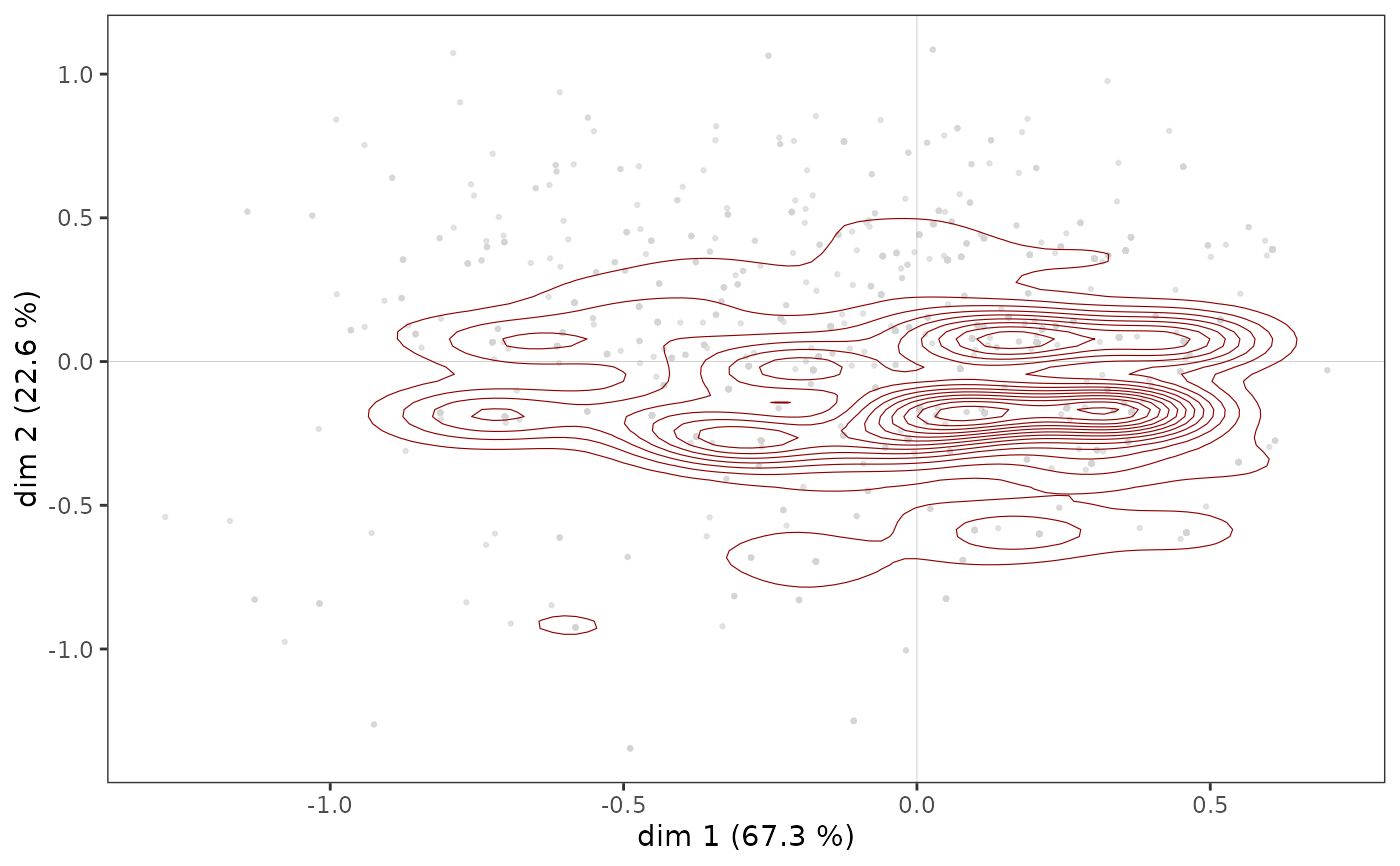
# density plot for Age = 50+ (with contours)
ggadd_density(p, mca, var = Taste$Age, cat = "50+")

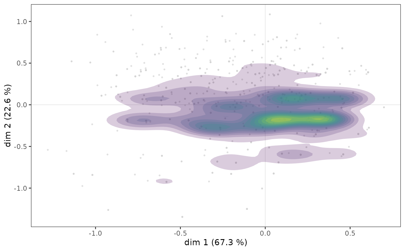
# density plot for Age = 50+ (with contours)
ggadd_density(p, mca, var = Taste$Age, cat = "50+", density = "area")