Plots the density a supplementary variable

Plots the density of a supplementary variable in a MCA space, using a grid, smoothing and interpolation (via inverse distance weighting.)

ggsmoothed_supvar(resmca, var, cat, axes = c(1,2), 
                  center = FALSE, scale = FALSE,
                  nc = c(20, 20), power = 2,
                  limits = NULL, pal = "RdBu")

Arguments

resmca

object of class PCA, MCA, speMCA, csMCA, stMCA or multiMCA.

var

factor or numeric vector. The supplementary variable to be plotted.

cat

character string. If var is a factor, the name of the level of the supplementary variable to be plotted.

axes

numeric vector of length 2, specifying the components (axes) to plot. Default is c(1,2).

center

logical. Whether the supplementary variable should be centered or not. Default is FALSE.

scale

logical. Whether the supplementary variable should be scaled to unit variance or not. Default is FALSE.

nc

integer vector of length 2. Number of grid cells in x and y direction (columns, rows).

power

numerical value. The power to use in weight calculation for inverse distance weighting. Default is 2.

limits

numerical vector of length 2. Lower and upper limit of the scale for the supplementary variable.

pal

character string. Name of a (preferably diverging) palette from the RColorBrewer package. Default is "RdBu".

Details

The construction of the plot takes place in several steps. First, the two-dimensional MCA space is cut into a grid of hexagonal cells. Then, for each cell, the average value of the supplementary variable is calculated for the observations located in that cell (if the variable is numerical), or the proportion of observations belonging to the category studied (if the variable is categorical). The results are interpolated and smoothed to make the plot easier to read, using the inverse distance weighting technique, which is very common in spatial analysis.

The supplementary variable can be centered beforehand, to represent deviations from the mean (for a numerical variable) or from the mean proportion (for a categorical variable). It can also be scaled to measure deviations in numbers of standard deviations, which can be useful for comparing the results of several supplementary variables.

Value

a ggplot2 object

References

Shepard, Donald (1968). "A two-dimensional interpolation function for irregularly-spaced data". Proceedings of the 1968 ACM National Conference. pp. 517–524. doi:10.1145/800186.810616

Author

Nicolas Robette

See also

ggadd_supvar, ggadd_supvars, ggadd_kellipses, ggadd_ellipses, ggadd_interaction, ggadd_corr, ggadd_chulls, ggadd_density

Examples

# specific MCA of Taste example data set
data(Taste)
junk <- c("FrenchPop.NA", "Rap.NA", "Rock.NA", "Jazz.NA", "Classical.NA",
          "Comedy.NA", "Crime.NA", "Animation.NA", "SciFi.NA", "Love.NA", 
          "Musical.NA")
mca <- speMCA(Taste[,1:11], excl = junk)
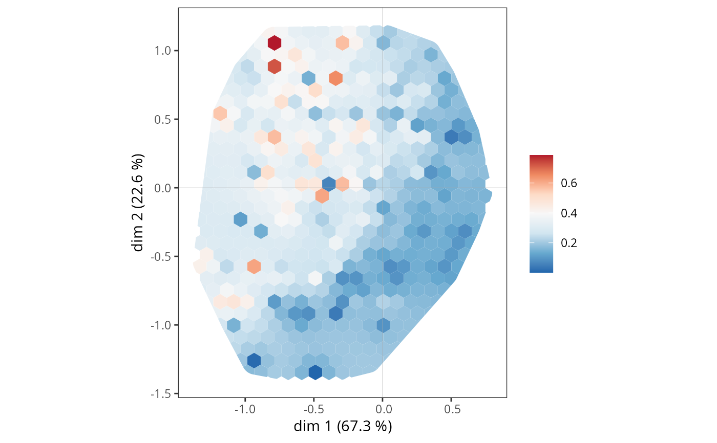
# density plot for Educ = "High"
ggsmoothed_supvar(mca, Taste$Educ, "High")

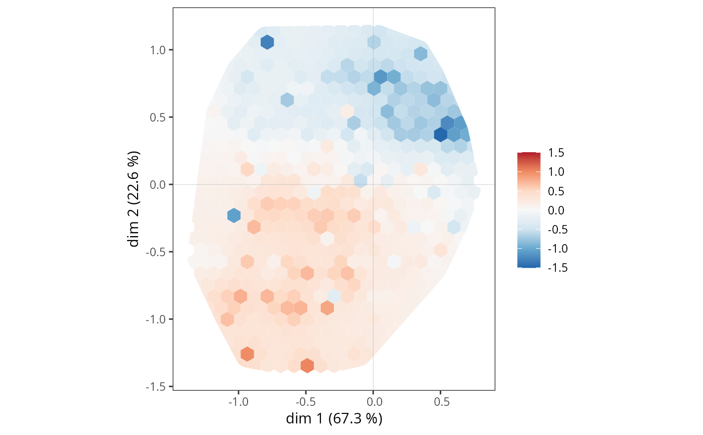
# centered and scaled density plot for Age
ggsmoothed_supvar(mca, as.numeric(Taste$Age), center = TRUE, scale = TRUE)