Principal Component Analysis with Instrumental Variables

Principal Component Analysis with Instrumental Variables

PCAiv(Y, X, row.w = NULL, ncp = 5)

Arguments

Y

data frame with only numeric variables

X

data frame of instrumental variables, which can be numeric or factors. It must have the same number of rows as Y.

row.w

Numeric vector of row weights. If NULL (default), a vector of 1 for uniform row weights is used.

ncp

number of dimensions kept in the results (by default 5)

Details

Principal Component Analysis with Instrumental Variables consists in two steps : 1. Computation of one linear regression for each variable in Y, with this variable as response and all variables in X as explanatory variables. 2. Principal Component Analysis of the set of predicted values from the regressions in 1 ("Y hat").

Principal Component Analysis with Instrumental Variables is also known as "redundancy analysis"

Value

An object of class PCA from FactoMineR package, with X as supplementary variables, and an additional item :

ratio

the share of inertia explained by the instrumental variables

.

References

Bry X., 1996, Analyses factorielles multiples, Economica.

Lebart L., Morineau A. et Warwick K., 1984, Multivariate Descriptive Statistical Analysis, John Wiley and sons, New-York.)

Author

Nicolas Robette

See also

bcPCA, DA, bcMCA, DAQ, MCAiv

Examples

library(FactoMineR)
data(decathlon)
# PCAiv of decathlon data set
# with Points and Competition as instrumental variables
pcaiv <- PCAiv(decathlon[,1:10], decathlon[,12:13])
pcaiv$ratio
#> [1] 0.3334462
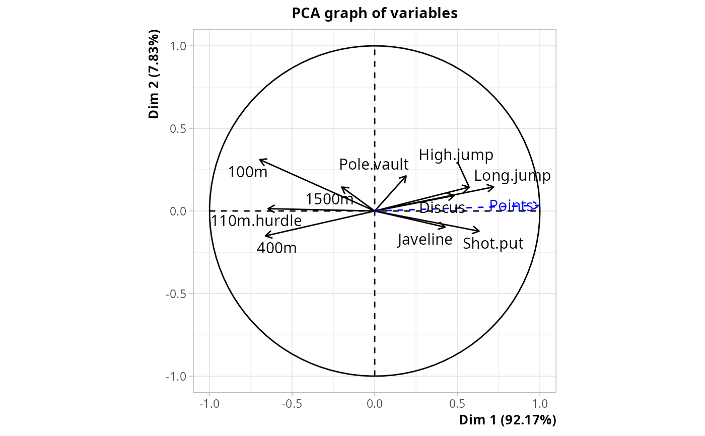
# plot of \code{Y} variables + quantitative instrumental variables (here Points)
plot(pcaiv, choix = "var")

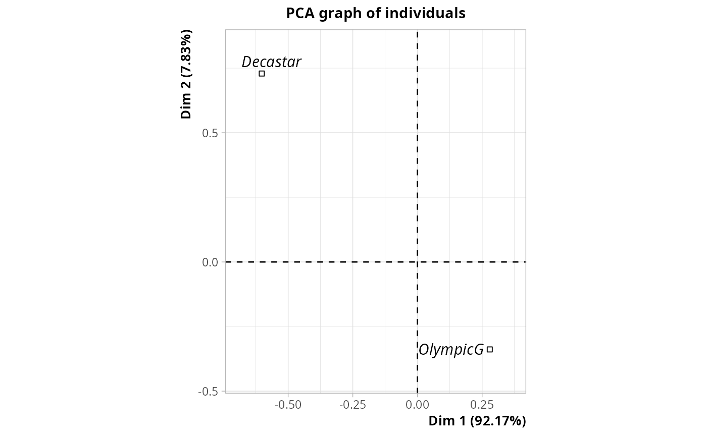
# plot of qualitative instrumental variables (here Competition)
plot(pcaiv, choix = "ind", invisible = "ind", col.quali = "black")