Multiple Correspondence Analysis with Instrumental Variables

Multiple Correspondence Analysis with Instrumental Variables

MCAiv(Y, X, excl = NULL, row.w = NULL, ncp = 5)

Arguments

Y

data frame with only factors

X

data frame of instrumental variables, which can be numeric or factors. It must have the same number of rows as Y.

excl

numeric vector indicating the indexes of the "junk" categories (default is NULL). See getindexcat or use ijunk interactive function to identify these indexes. It may also be a character vector of junk categories, specified in the form "namevariable.namecategory" (for instance "gender.male").

row.w

Numeric vector of row weights. If NULL (default), a vector of 1 for uniform row weights is used.

ncp

number of dimensions kept in the results (by default 5)

Details

Multiple Correspondence Analysis with Instrumental Variables consists in three steps : 1. Specific MCA of Y, keeping all the dimensions of the space 2. Computation of one linear regression for each dimension in the specific MCA, with individual coordinates as response and all variables in X as explanatory variables. 3. Principal Component Analysis of the set of predicted values from the regressions in 2.

Multiple Correspondence Analysis with Instrumental Variables is also known as "Canonical Correspondence Analysis" or "Constrained Correspondence Analysis".

Note

If there are NAs in Y, these NAs will be automatically considered as junk categories. If one desires more flexibility, Y should be recoded to add explicit factor levels for NAs and then excl option may be used to select the junk categories.

Value

An object of class PCA from FactoMineR package, with Y and X as supplementary variables, and an additional item :

ratio

the share of inertia explained by the instrumental variables

.

References

Bry X., 1996, Analyses factorielles multiples, Economica.

Lebart L., Morineau A. et Warwick K., 1984, Multivariate Descriptive Statistical Analysis, John Wiley and sons, New-York.)

Author

Nicolas Robette

See also

bcMCA, DAQ, bcPCA, DA, PCAiv

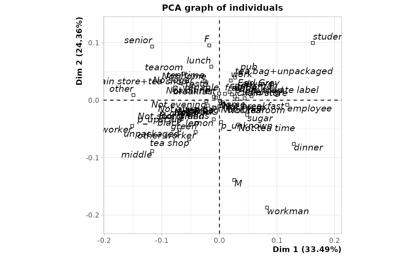
Examples

library(FactoMineR)
data(tea)
# MCAIV of tea data
# with age, sex, SPC and Sport as instrumental variables
mcaiv <- MCAiv(tea[,1:18], tea[,19:22])
mcaiv$ratio
#> [1] 0.05709817
plot(mcaiv, choix = "ind", invisible = "ind", col.quali = "black")