Plot of correlations
plo_cor.RdPlots the correlations between (X and Y) variables and the components (X scores) of a PLS regression.
plo_cor(object, comps = 1:2, which = "both", min.cor = NULL,
        lim = NULL, circles = NULL, col = NULL, size = 3.88)
Arguments
- object
an object of class
mvrfromplspackage- comps
the components to use. Default is
c(1,2).- which
character string. If
"both"(default), X and Y variables are plotted. If"X", only X variables are plotted. If"Y", only Y variables are plotted.- min.cor
numerical value. The minimal correlation with one or the other component for a variable to be plotted. If
NULL(default), all the variables are plotted.- lim
numerical value. The limit of the scale (in absolute value). If
NULL(default), the limits are automatically determined from the range of tha data.- circles
vector of numeric values. Circles are added to the plot at radiuses specified in
circles. IfNULL(default), no circle is plotted.- col
colors for the names of the variables. Only one value should be provided if
whichis "X" or "Y", a vector of two ifwhichis "both". IfNULL(default), colors are set automatically.- size
numerical value. The size of the names of the variables.
Value
a ggplot2 object
Note
This is what Tenenhaus calls the univariate interpretation of the PLS components, as opposed to the multivariate interpretation (see plo_var).
References
Martens, H., Næs, T. (1989) Multivariate calibration. Chichester: Wiley.
Tenenhaus, M. (1998) La Regression PLS. Theorie et Pratique. Editions TECHNIP, Paris.
Examples
library(pls)
data(yarn)
pls <- mvr(density ~ NIR,
ncomp = 5,
data = yarn,
validation = "CV",
method = "oscorespls")
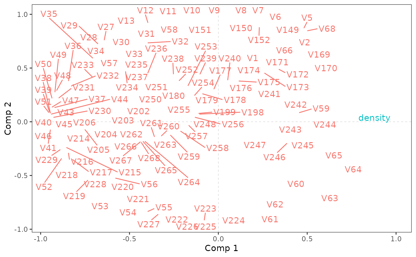
plo_cor(pls)
#> Warning: ggrepel: 128 unlabeled data points (too many overlaps). Consider increasing max.overlaps
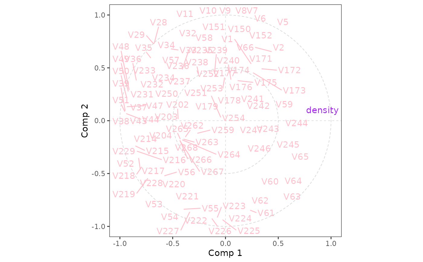
 # plot with circles corresponding to
# correlations of 0.5 and 1
plo_cor(pls, lim = 1, circles = c(0.5, 1), col = c("pink", "purple"))
#> Warning: ggrepel: 131 unlabeled data points (too many overlaps). Consider increasing max.overlaps
# plot with circles corresponding to
# correlations of 0.5 and 1
plo_cor(pls, lim = 1, circles = c(0.5, 1), col = c("pink", "purple"))
#> Warning: ggrepel: 131 unlabeled data points (too many overlaps). Consider increasing max.overlaps